EMNLP2024 论文研读 - 参数高效稀疏化

论文：Parameter-Efficient Sparsity Crafting from Dense to Mixture-of-Experts for Instruction Tuning on General Tasks

摘要

Large language models (LLMs) have demon-strated considerable proficiency in general natural language processing(NLP) tasks. Instruc-tion tuning, a successful paradigm, enhances the ability of LLMs to follow natural language instructions and exhibit robust generalization across general tasks. However, these models often encounter performance limitations across multiple tasks due to constrained model capacity. Expanding this capacity during the in-struction tuning phase poses significant challenges. To address this issue, we introduce parameter-efficient sparsity crafting (PESC), which crafts dense models into sparse models using the mixture-of-experts (MoE) architec-ture. PESC integrates adapters into the MoE layers of sparse models, differentiating experts without altering the individual weights within these layers. This method significantly reduces computational costs and GPU memory require-ments, facilitating model capacity expansion through a minimal parameter increase when guaranteeing the quality of approximation in function space compared to original sparse up-cycling. Our empirical evaluation demonstrates the effectiveness of the PESC method. Using PESC during instruction tuning, our best sparse model outperforms other sparse and dense models and exhibits superior general capabilities compared to GPT-3.5. Our code is available at https://github.com/wuhy68/Parameter-Efficient-MoE.

这篇论文主要介绍了一种名为 PESC 的新方法，用于解决大型语言模型在指令微调过程中的容量限制问题。该方法通过 MoE 架构将密集模型转化为稀疏模型，并创新性地使用适配器（Adapters）来区分专家，而无需改变这些层的内部权重。这种方法不仅降低了计算和内存开销，还能在最小化参数增加的情况下有效扩展模型容量。实验结果表明，使用 PESC 方法训练的稀疏模型在性能上超过了其他模型，包括 GPT-3.5，证明了该方法的实用价值和效果。

引言

作者指出，训练 LLM 的一个显著方法是指令调优（Instruction Tuning），这种方式通过使用大规模、格式良好的指令数据训练 LLM，使 LLM 能够优化其预训练表示以符合人类指令，然而，这些任务固有的复杂性可能会阻碍模型微调，具体来说，某些规模的模型可能难以从冲突的任务中优化损失，导致通用任务的表现不佳。

The Scaling Law 表明增加模型的规模对提高模型表现至关重要，扩大模型的容量也可以提高对通用任务指令微调的有效性，然而，大多数 LLM 都是基于 Transformer 架构设计的预训练密集模型（dense model），这限制了指令微调过程中的可扩展性。Komatsuzaki et al.(2023) 提出了一种将密集模型改造为稀疏激活的 MoE 模型 的方法，并使模型具有了更大的容量；Shen et al.(2023) 指出与密集模型相比，MoE 模型对指令微调的响应更加有效，因此，在指令微调时将密集模型转换成 MoE 模型有可能在一般任务上取得优异表现。但是鉴于当前 LLM 的参数规模，训练这样的巨型模型需要更新 MoE 层中专家的权重，这受到 GPU 内存资源和计算成本的制约。

从以上描述可知，作者主要关注的问题是：

1. 将密集模型拓展到稀疏 MoE 模型以增大模型容量（增大模型容量可能带来提升效果；拓展为 MoE 模型可能对指令微调的响应更佳）

2. 对 MoE 模型进行指令微调时，更新各专家的权重，会占用大量计算与内存资源（如何高效微调）

作者提出了参数高效稀疏化构建（PESC）的方法，在有效拓展模型容量的同时能与 PEFT 协同工作。对于第一个问题，其实先前也有类似的解决方案，见论文 Sparse Upcycling: Training Mixture-of-Experts from Dense Checkpoints，而该篇论文在稀疏化构建的方法上很相似，我们可以对比两者的结构示意图：

Sparse Upcycling：

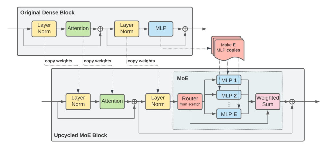
本文：

其主要的改进部分是在稀疏化后的 MoE 层中，在 FFN 的上面添加了 Adapters 适配层以利用 PEFT 的思路进行稀疏化后的训练，后面将详细分析。

方法论

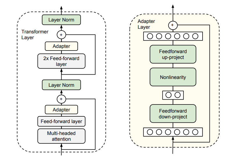
Adapters

首先介绍 Houlsby et al.(2019) 提出的一种将适配器集成到 Transformer-based 的预训练模型中的参数高效微调方法，这种方法只需要调整添加的 adapter 层的参数即可，一个适配器包括两个矩阵： $W{down} \in \mathbb{R}^{d_1 \times d_2}$ 和 $W{up} \in \mathbb{R}^{d_2 \times d_1}$，再加上一个非线性函数（激活函数），其中 $d_1$ 和 $d_2$ 分别表示预训练模型的特征维度（hidden_size）和适配器的隐藏维度（adapter hidden size），一般来说 $d_2 < d_1$，给出预训练模型的特征 $U \in \mathbb{R}^{N \times d_1}$，适配器模块的输出为：

$$U' = \sigma\left( UW_{dowm} \right)W_{up} + U$$

我们来看一下在 Adapter 原论文中的介绍的高效微调方法，从图片中我们也可以直观的理解其计算过程：

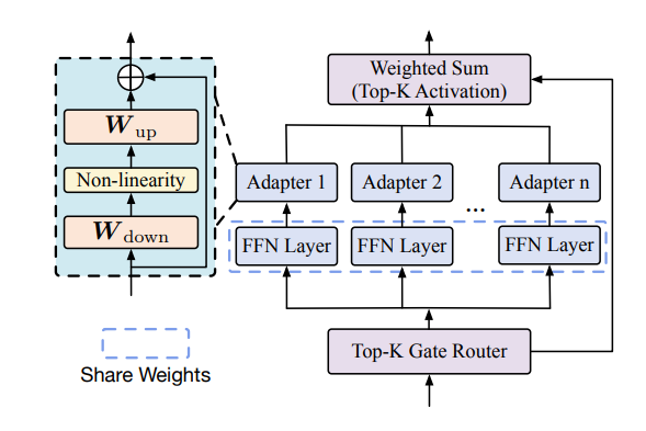
在该论文中使用的 Adapter 与上图中的方法基本是一样的，该论文中具体的 MoE 层设计如下图所示：

Mixture-of-Experts

一个经典的专家混合的输出设计为（具体可参见论文Outrageously Large Neural Networks: The Sparsely-Gated Mixture-of-Experts Layer，相关研读The Sparsely-Gated Mixture-of-Experts Layer 论文研读 | Relativity suis’s Blog）：

$$y = \sum_{i=1}^n R(x)_iE_i(x) \tag{1}$$

其中 $R(x)$ 是门控网络的输出（筛选出真正要使用的专家，首先经过 $\texttt{KeepTopK}$ 筛选出前 $K$ 个专家，然后使用 $\texttt{softmax}$ 归一化生成权重），$E_i(x)$ 是第 $i$ 个专家的输出。

Sparsity Crafting

基于 Sparse Upcycling 的工作，其核心是利用原密集模型的权重，并涉及到一个变革性的过程：在原密集 Transformer 模型的每个 block 中，用 MoE 层替换 FFN 层，在稀疏性构建的初始化阶段，使用原密集模型的 FFN 的权重作为 MoE 层中每个专家的 FFN 模块的初始化权重，Adapter 层的权重为随机初始化，同时，为了确保结构的一致性，模型中的其他模块（如 Attention 层和 Norm 层等）直接从原模型中 copy 过来，现在再看模型的结构图我们也可以更好地理解。

参数高效的稀疏性构建

我们再仔细来看 Sparse Upcycling 中的稀疏性构建与训练过程，主要关注 MoE 层，在这篇工作里的作者将 MoE 层的所有专家设计为 MLP，初始化为对应 block 的 FFN 层的参数，因此在后面的训练过程中需要更新的参数就是所有块的所有专家（即 MLP）的所有参数，这其实就会造成大量的参数更新，从而需要很多的计算与存储资源，并导致训练时间变长（并不高效）。

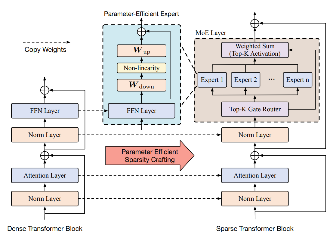
而本文中作者来改善 / 缓解这一问题的方法就是，在专家的 FFN / MLP（本文中作者称为 FFN。其实都差不多）上添加 Adapters 适配器层，从而只需要通过更新适配器层的少量参数即可达成训练的目的（效果与前面的方法相比在可接受范围内，也就类似于全量微调与参数高效微调的关系），实际上也就是利用了 PEFT 的思想与方法，后面作者通过一些数学解释与文献引用，也说明了使用适配器的方法能够有效地保证近似质量（与专家参数全调整相比）。

我们可以再来对比两者的结构示意图，主要区别就在于专家层里：

Sparse Upcycling：

本文：

模型设计

经过上述分析，我们可以更新方程 1 的表示：

$$y = \sum_{i=1}^n R(x)_iA_i(E(x))$$ $$A_i(x) = \sigma(xW_{i_{down}})W_{i_{up}} + x$$

这样我们更新的参数就不是整个 $Ei(x)$ ，而是适配器的参数 $W{i{down}},~W{i_{up}}$

门控网络的设计没有什么变化：

$$R(x) = \texttt{softmax}(\texttt{KeepTopK}(W_{route} \cdot x))$$

对于负载均衡，论文中描述：

Top-K 门控路由器通过其门控机制，往往会不成比例地偏 向某几个专家，导致这些专家更频繁地被训练和被路由器选择，为了解决这种不平衡并促进专家的均匀使用，我们在每个稀疏 Transformer 块的训练过程中引入了一个辅助损失函数（由 Fedus 等人(2022)提出）。对于 $n$ 个专家和包含 $T$ 个 token 的批次 $B$，专家负载均衡的辅助损失 $\mathcal{L}$ 计算为向量 $f$ 和 $p$ 的缩放点积：
数学公式：

$$\mathcal{L} = \alpha \cdot n \cdot \sum_{i=1}^n f_i \cdot p_i$$

其中 $f_i$ 表示分配给专家 $i$ 的 token 比例，$p_i$ 表示分配给专家i的路由概率比例。$\alpha$ 是辅助损失的乘性系数，我们使用 $\alpha = 10^{-2}$，这个值足够大以确保负载均衡，同时又足够小以不会压倒主要的交叉熵目标。理想情况下，应该在 $n$ 个专家之间实现均匀路由，因此两个向量的理想值都应该是 $\frac{1}{n}$，上述方程中的辅助损失促进了这种均匀分布，并在这种条件下达到最小值。

代码实现

模型构建

在该篇工作中，模型实现的重点就是对模型从密集变换成稀疏模型的部分，与添加 Adapters 层的部分，在本文的代码仓库中主要在 ./camelidae/modeling_camelidae.py 中实现，我们看其中的一部分：

class ParallelAdapterMLP(nn.Module):
    def __init__(self, config, adapter_dim, adapter_scaling):
        super().__init__()
        self.config = config
        self.intermediate_size = config.intermediate_size
        self.hidden_size = config.hidden_size
        self.adapter_down = nn.Linear(self.hidden_size, adapter_dim, bias=False)
        self.adapter_up = nn.Linear(adapter_dim, self.hidden_size, bias=False)
        self.adapter_act = nn.GELU()

        self.adapter_dropout = nn.Dropout(p=0.1)
        self.adapter_scaling = adapter_scaling

    def forward(self, x):
        x = self.adapter_dropout(x)
        x = self.adapter_scaling * self.adapter_up(self.adapter_act(self.adapter_down(x)))
        return x


class CamelidaeGateAdapter(nn.Module):
    def __init__(self, config: CamelidaeConfig):
        super().__init__()

        self.intermediate_size = config.intermediate_size
        self.hidden_size = config.hidden_size

        # Step 1: Router
        self.num_experts = config.num_experts
        self.topk = config.topk
        self.router = nn.Linear(
            config.hidden_size, self.num_experts, bias=False
        )
        self.dtype = getattr(torch, config.moe_dtype)

        # Step 2: Get the experts
        self.experts = nn.ModuleDict()
        for idx in range(config.num_experts):
            self.experts[f"expert_{idx}"] = ParallelAdapterMLP(config, config.adapter_dim, config.moe_scaling)
            
    def forward(self, input_hidden_states, output_hidden_states, router_hidden_states):
        orig_shape = output_hidden_states.shape
        input_hidden_states = input_hidden_states.view(-1, input_hidden_states.shape[-1])
        output_hidden_states = output_hidden_states.view(-1, output_hidden_states.shape[-1])
        router_hidden_states = router_hidden_states.view(-1, router_hidden_states.shape[-1])

        router_logits = self.router(router_hidden_states)

        expert_weights, expert_indices = torch.topk(router_logits, self.topk, dim=-1)
        expert_weights = expert_weights.softmax(dim=-1)
        flat_expert_indices = expert_indices.view(-1)

        input_hidden_states = input_hidden_states.repeat_interleave(self.topk, dim=0)
        expert_hidden_states = output_hidden_states.repeat_interleave(self.topk, dim=0)
        for idx, expert in enumerate(self.experts.values()):
            expert_hidden_states[flat_expert_indices == idx] += expert(input_hidden_states[flat_expert_indices == idx])
        hidden_states = (expert_hidden_states.view(*expert_weights.shape, -1) * expert_weights.unsqueeze(-1)).sum(dim=1)

        return hidden_states.view(*orig_shape), router_logits

ParallelAdapterMLP 类构建了添加到专家 FFN 后的适配器层，可以看到其 forward 方法与前面叙述的一致，然后在 CamelidaeGateAdapter 类中调用了该类，为每个专家添加一个适配器，在CamelidaeGateAdapter 类的 forward 中也可以看到 MoE 层中从输入门控网络得到输出分布，后经过 KeepTopK 和 softmax 操作得到门控的输出 $R(x)$，与处理专家的输入输出的过程。

QLoRA

另外作者提到，在本文的研究中，对于 MoE 层的专家通过添加 Adapters 层进行微调，然后使用 QLoRA 对其他层进行微调，在 train_moe.py 中我们关注 train 函数，可以看到：

def train():
    parser = transformers.HfArgumentParser(
        (ModelArguments, DataArguments, TrainingArguments)
    )
    model_args, data_args, training_args = parser.parse_args_into_dataclasses()
    training_args.ddp_find_unused_parameters = False
    set_seed(42)

    model_config = CamelidaeConfig.from_pretrained(model_args.model_name_or_path)
    model_config.pretraining_tp = 1  ## without tensor parallelism rank

    # Camelidae Config
    model_config.moe_dtype = "bfloat16"
    model_config.lora_r = 64
    model_config.lora_alpha = 16
    model_config.adapter_dim = 64
    model_config.topk = 2
    model_config.moe_scaling = 1
    model_config.num_experts = 8
    model_config.output_router_logits = False

    # # Seq Length Extension
    # model_config.rope_scaling = {
    #     "type": "dynamic",
    #     "factor": 2,
    # }

    model = LlamaForCausalLM.from_pretrained(
        model_args.model_name_or_path,
        config=model_config,
        cache_dir=training_args.cache_dir,
        load_in_4bit=True,
        quantization_config=BitsAndBytesConfig(
            load_in_4bit=True,
            bnb_4bit_compute_dtype=torch.bfloat16,
            bnb_4bit_use_double_quant=True,
            bnb_4bit_quant_type="nf4",
        ),
        output_loading_info=False,
    )
    model = prepare_model_for_kbit_training(model, use_gradient_checkpointing=True)
    model.gradient_checkpointing_enable()

    # lora_modules = find_all_linear_names(model)
    lora_modules = [
        "q_proj",
        "k_proj",
        "v_proj",
        "o_proj",
        "up_proj",
        "gate_proj",
        "down_proj",
    ]
    config = LoraConfig(
        r=model_config.lora_r,
        lora_alpha=model_config.lora_alpha,
        target_modules=lora_modules,
        lora_dropout=0.1,
        bias="none",
        task_type="CAUSAL_LM",
    )
    model = get_peft_model(model, config)

    # Zero Init
    for n, p in model.named_parameters():
        if "adapter_up" in n:
            nn.init.zeros_(p)
        if "adapter_down" in n:
            nn.init.kaiming_uniform_(p, a=math.sqrt(5))
        if "router" in n:
            nn.init.kaiming_uniform_(p, a=math.sqrt(5))

    for name, module in model.named_modules():
        if isinstance(module, LoraLayer):
            if training_args.bf16:
                module = module.to(torch.bfloat16)
        if "norm" in name:
            module = module.to(torch.float32)
        if "lm_head" in name or "embed_tokens" in name:
            if hasattr(module, "weight"):
                if training_args.bf16 and module.weight.dtype == torch.float32:
                    module = module.to(torch.bfloat16)
        if "adapter" in name:
            if training_args.bf16:
                module = module.to(torch.bfloat16)
            else:
                module = module.to(torch.float32)

    for n, p in model.named_parameters():
        if "adapter" in n:
            p.requires_grad = True
        # if "norm" in n:
        #     p.requires_grad = True

    model.config.use_cache = False
    print_trainable_parameters(model)

    tokenizer = transformers.AutoTokenizer.from_pretrained(
        model_args.model_name_or_path,
        cache_dir=training_args.cache_dir,
        model_max_length=training_args.model_max_length,
        padding_side="right",
        use_fast=False,
        trust_remote_code=True,
    )
    if tokenizer.pad_token is None:
        tokenizer.pad_token_id = (
            0  # unk. we want this to be different from the eos token
        )

    data_module = make_supervised_data_module(tokenizer=tokenizer, data_args=data_args)
    trainer = Trainer(
        model=model, tokenizer=tokenizer, args=training_args, **data_module
    )
    trainer.add_callback(SavePeftModelCallback)

    trainer.train()

    model.save_pretrained(training_args.output_dir)

其中：

model = LlamaForCausalLM.from_pretrained(
    model_args.model_name_or_path,
    config=model_config,
    cache_dir=training_args.cache_dir,
    load_in_4bit=True,
    quantization_config=BitsAndBytesConfig(
        load_in_4bit=True,
        bnb_4bit_compute_dtype=torch.bfloat16,
        bnb_4bit_use_double_quant=True,
        bnb_4bit_quant_type="nf4",
    ),
    output_loading_info=False,
)
model = prepare_model_for_kbit_training(model, use_gradient_checkpointing=True)
model.gradient_checkpointing_enable()

# lora_modules = find_all_linear_names(model)
lora_modules = [
    "q_proj",
    "k_proj",
    "v_proj",
    "o_proj",
    "up_proj",
    "gate_proj",
    "down_proj",
]

是一些量化的配置与使用 LoRA 模块微调的模块，可以看到一共调整了注意力模块中的 qkvo 投影矩阵，门控矩阵与 MoE 层中的 FFN 模块，也就是说调整了除添加的 Adapters 的所有权重矩阵。

其他

作者还探讨了关于 Mixture of LoRA Experts 的相关内容，先在这里把翻译过来的部分贴出来：

其他研究也探讨了将混合专家模型（MoE）与参数高效微调技术（PEFT）相结合的方法（Diao等，2023；Gou等，2023；Wu等，2024b；Liu等，2023；Luo等，2024；Dou等，2024）。例如，LoRAMoE（Dou等，2024）专注于世界知识的保留，而 MoELoRA（Luo等，2024）则利用统一了 MoE 和 LoRA 的 PEFT 框架，专注于数学和常识推理能力。然而，LoRA 框架的混合在训练和推理过程中带来了额外的计算成本，包括更高的内存占用和在没有并行化的情况下速度较慢。相比之下，我们的 PESC 方法则不会面临这些挑战。PESC 基于适配器模型框架，通过在复制的 FFN 层后插入多个适配器进行微调，而不是在相应的专家中微调所有复制的 FFN 层。在我们的 PESC 的 MoE 设计中，每个专家使用单一的适配器模块，与 LoRA 模块相比，显著减少了整体内存占用，因为 LoRA 模块由于其在 FFN 和注意力层中的位置，每个专家需要多个模块。这一区别在处理大量专家时尤为重要，因为内存限制变得越来越具有挑战性。此外，我们基于适配器的专家设计使得专家之间能够并行计算，因为它们彼此的输出相互独立，这与 LoRA 不同，LoRA 中层级之间的依赖关系可能会限制并行性。这种设计加速了训练时间，尤其是在专家数量增加的情况下，确保了可扩展性和效率。还值得注意的是，LoRA 在推理时可能需要将权重合并到主模型中，导致内存使用增加和潜在的延迟问题，特别是当多个令牌激活不同的专家时。相反，基于适配器的参数高效 MoE 在推理时不会产生这种开销，保持了与原始密集模型相似的低计算负担。

这里其实没有太看明白作者是在拿自己的方法跟具体怎样使用 LoRA 的结果进行对比，不过作者前面提到了 LoRAMoE 和 MoELoRA 的工作，我们也先来看看：

LoRAMoE：

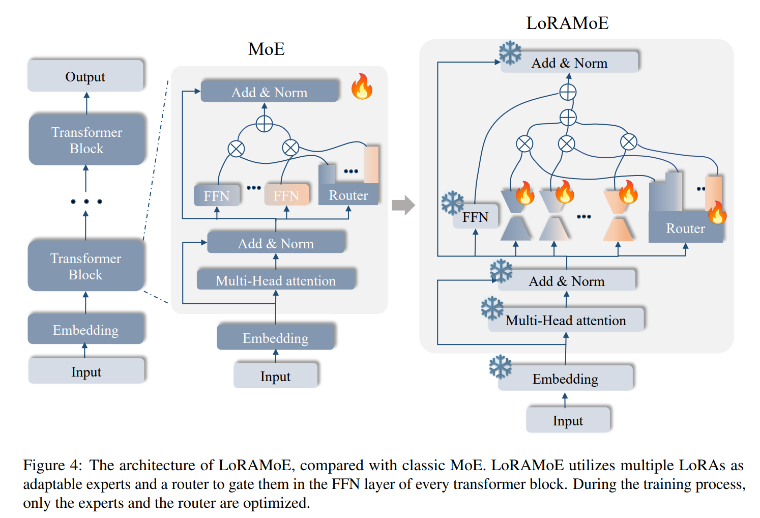
从示意图中可以很清楚地看出模型的工作原理，将原模型的其他模块迁移到 LoRAMoE 结构中，并保持参数冻结（包括 FFN 层），然后将 LoRA 模块视为 MoE 层的所有专家，通过门控网络控制专家的输出，再与 FFN 的输出相加。简单来说也就是冻结主干模型，引入多个 LoRA 适配器，使用路由网络（门控）整合这些适配器

MoELoRA：

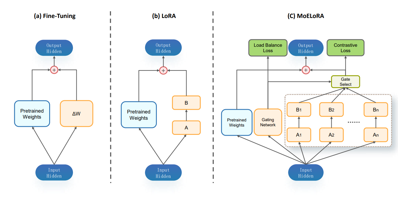
MoELoRA 则是将 LoRA 视为一个专家系统，我们可以最后做一个对比：

1. 该篇工作（PESC）的设计与 LoRAMoE 的设计具有一些相似之处，其都保持了 Norm 和 Attention 等层的参数不变（冻结），而专注于处理 MoE 层的变化，PESC将 Transformer Block 中的 FFN 复制为 $N$ 份，作为 $N$ 个专家的 FFN 层的初始化，然后在这些 FFN 层后添加 Adapters 适配器层；LoRAMoE 则是将 Transformer Block 中的 FFN 保持冻结，同时使用若干 LoRA 模块作为专家使用，最后将专家（经门控）的输出与 FFN 的输出结合得到最终结果。
2. MoELoRA 则是将 LoRA 本身视为专家系统，将这一原本用于微调的 LoRA 模块改变为由 LoRA 模块组成的专家系统。